Fundamentals of steel deoxidation

Fundamentals of steel deoxidation#

Dr. Edgar Ivan Castro Cedeño

import numpy as np
import pandas as pd
import matplotlib.pyplot as plt
from scipy.optimize import fsolve

import warnings
warnings.filterwarnings('ignore')

Metallurgical context#

At the end of the primary steelmaking process (BOF/EAF), the liquid steel contains high amount of dissolved oxygen. The order of magnitude for the amount of oxygen is:

\[a_O > 300 \, ppm\]

Hence, one of the steps in the secondary refining of steel is steel deoxidation. The deoxidation of the liquid steel bath can be carried out by means of the addition of deoxidizing agents or by vacuum treatment.

The intent of this document is to review basic concepts of steel deoxidation carried out by addition of deoxidizing agents, and applying them to the process of secondary refining of steels.

Generalized deoxidation reaction#

In a general form, the steel deoxidation reaction can be expressed as:

\[\left(M_xO_y\right) = x\left[M\right] + y\left[O_x\right] \]

\[K = \frac{a_M^x a_O^y}{a_{M_xO_y}} \]

where \(a_{M_xO_y}\), \(a_M^x\), y \(a_O^y\), are the thermodynamic activities of the chemical species of interest.

Reference states#

For the deoxidation products the pure-substance is used as reference state:

\[a_{M_xO_y} = \gamma_{M_xO_y} {X_{M_xO_y}} \]

Symbol	Description
\(a_{M_xO_y}\)	Activity of the deoxidation product \(M_xO_y\)
\(\gamma_{M_xO_y}\)	Raoultian activity coefficient
\(X_{M_xO_y}\)	Contents of the \(M_xO_y\) species in the deoxidation product, in molar fraction

This document does not discuss about methods for estimating the activity of deoxidation products in complex systems.

For the solutes in the liquid metal bath the Henrian 1% mass dilution is used as reference state:

\[h_M = f_M {\left[\%M\right]} \]

Symbol	Description
\(h_M\)	Activity of the solute \(M\)
\(f_M\)	Henrian activity coefficient
\(\left[ \%M \right]\)	Contents of solute \(M\) in the bath, in mass percent

Wagner Formalism (Interaction coefficients)#

The Wagener formalism of interaction coefficients will be used in order to consider the dependencies between bath composition and the thermodynamic activity of the solutes.

\[\log f_i = \sum\limits_{j=2}^{n}{e_i^j \left[\%j\right]} + \sum\limits_{j=2}^n{r_i^j \left[ \%j\right]^2} + \sum\limits_{j=2}^{n-1} \sum\limits_{k>j}^{n} {r_i^{j,k} \left[\%j\right]\left[\%k\right]}\]

Symbol	Description
\(e_i^j\)	First order interaction coefficient for solute \(i\) in the presence of solute \(j\)
\(r_i^j\)	Second order interaction coefficient for solute \(i\) in the presence of solute \(j\)
\(r_i^{j,k}\)	Second order interaction coefficient for solute \(i\) in the presence of solutes \(j\), \(k\)

The Wagner formalism was originally proposed for the case of infinite dilution, however it has proveen that it can give reliable results for the treatment of solutions with “low” solute concentration, such as the case of iron and steel. The higher order interaction parameters are used for the cases of alloyed steels, in which the concentrations of solutes are higher.

Deoxidation with aluminium#

Alumina inclusion

Deoxidation reaction#

The deoxidation reaction by aluminium is given by:

\[\left( Al_{2}O_{3}\right) = 2 \left[Al\right] + 3 \left[O\right] \]

\[K_{Al} = \frac{h_{Al}^2 h_{O}^3}{a_{Al_2O_3}} \]

Where the aluminium activity is given by:

\(h_{Al} = f_{Al} [\%Al]\)

\(\log f_{Al} = e_{Al}^{Al} \left[\%Al\right] + e_{Al}^{O} \left[\%O\right] + r_{Al}^{Al,Al} \left[\%Al\right]^2 + r_{Al}^{O,O} \left[\%O\right]^2 + r_{Al}^{Al,O} \left[\%Al\right]\left[\%O\right] \)

and the oxygen activity is given by:

\(h_O = f_{O} [\%O]\)

\(\log f_{O} = e_{O}^{Al} \left[\%Al\right] + e_{O}^{O} \left[\%O\right] + r_{O}^{Al,Al} \left[\%Al\right]^2 + r_{O}^{O,O} \left[\%O\right]^2 + r_{O}^{Al,O} \left[\%Al\right]\left[\%O\right] \)

Numerical value for the equilibrium constant#

A recommended value for the deoxidation constant is given by:

\[\log K_{Al} = -\frac{45300}{T} + 11.62 \]

def logK_Al(T: float) -> float:
    """
    logarithm of equilibrium constant: Al-O
   
    Parameters
    ----------
    T : Float
        Temperature, in [K]
       
    Returns
        logarithm of equilibrium constant
    """
    return -45300 / T + 11.62

Numerical value for the interaction coefficients#

First order interaction coefficients#

\[\begin{split}\begin{bmatrix}e_{Al}^{Al} & e_{Al}^{O} \\ e_{O}^{Al} & e_{O}^{O}\end{bmatrix} = \begin{bmatrix}\frac{80.5}{T} & 3.21 - \frac{9720}{T} \\ 1.90 - \frac{5750}{T} & 0.76 - \frac{1750}{T}\end{bmatrix}\end{split}\]

def e_AlAl(T: float) -> float:
    return 80.5 / T

def e_AlO(T: float) -> float:
    return 3.21 - 9720 / T

def e_OAl(T: float) -> float:
    return 1.90 - 5750 / T

def e_OO(T: float) -> float:
    return 0.76 - 1750/T

Second order interaction coefficients#

\[\begin{split}\begin{bmatrix}r_{Al}^{Al, Al} & r_{Al}^{O,O} \\ r_{O}^{Al, Al} & r_{O}^{O,O}\end{bmatrix} = \begin{bmatrix}0 & -107 - \frac{2.75\times10^{5}}{T} \\ 0.0033 - \frac{25.0}{T} & 0\end{bmatrix}\end{split}\]

\[\begin{split}\begin{bmatrix} r_{Al}^{Al, O} \\ r_{O}^{Al, O}\end{bmatrix} = \begin{bmatrix} -0.021 - \frac{13.78}{T} \\ 127.3 + \frac{3.273\times10^{5}}{T} \end{bmatrix}\end{split}\]

def r_AlAl(T: float) -> float:
    return 0

def r_AlO(T: float) -> float:
    return -107 - 2.75e5 / T

def r_OAl(T: float) -> float:
    return 0.0033 - 25 / T

def r_OO(T: float) -> float:
    return 0

def r_AlAlO(T: float) -> float:
    return -0.021 -13.78 / T

def r_OAlO(T: float) -> float:
    return 127.3 + 3.273e5 / T

Construction of equilibrium curves for deoxidation with aluminium#

Numerical method#

Applying logarithm laws, the equilibrium constant and the deoxidation reaction can be rewritten as:

\[\log K_{Al} = 2 \log f_{Al} + 2 \log \left[\%Al\right] + 3 \log f_{O} + 3 \log \left[\%O \right] - \log a_{Al_2O_3} \]

In the function Al_o_eqs the equation shown above is rewritten so that when the root of the equation is calculated by a numerical method, the combinations of dissolved aluminium and oxygen contents that satisfy the thermodynamic equilibrium constraints can be determined.

\[\varepsilon = 2 \log f_{Al} + 2 \log \left[\%Al\right] + 3 \log f_{O} + 3 \log \left[\%O \right] - \log a_{Al_2O_3} - \log K_{Al}\]

def Al_O_eqs(pctO: float, *params) ->float:
    """
    remainder of Thermodynamic equilibrium equation: Al-O
    Activity coefficients calculated with none, only first order, or
    first and second order interaction coefficients
    
    Parameters
    ----------
    pctO : Float
        weight percent oxygen.
    *params : List or tupples
        pctAl: weight percent aluminum (float)    
        T: Temperature in K (float)
        aAl2O3: thermodynamic activity of Al2O3 (float)
        order: 0: no interacion params., 1: e_ij, 2: e_ij, r_ij, r_ijk (integer)
        
    Returns
    -------
    eps : float
        LHS residual of the equation.
    """
    pctAl, T, aAl2O3, order = params # unpacking of parameters

    log_K = logK_Al(T)
    log_aAl2O3 = np.log10(aAl2O3)
        
    if order == 0:
        log_fAl = 0
        log_fO  = 0
    elif (order == 1 or order ==2):
        log_fAl = e_AlAl(T)*pctAl + e_AlO(T)*pctO
        log_fO  = e_OAl(T)*pctAl + e_OO(T)*pctO
        if order == 2:
            log_fAl += r_AlAl(T)*pctAl**2 + r_AlO(T)*pctO**2 + r_AlAlO(T)*pctAl*pctO
            log_fO  += r_OAl(T)*pctAl**2 + r_OO(T)*pctO**2 + r_OAlO(T)*pctAl*pctO
    else:
        valid = [0, 1, 2]
        raise ValueError(f"order: {order} is not a valid integer, choose either {valid }")
        
    eps = 2*log_fAl + 2*np.log10(pctAl) + 3*log_fO + 3*np.log10(pctO) - log_aAl2O3 - log_K
    
    return eps

The functions calc_pure() and data_deox() are wrappers for using the fsolve() function from the scipy.optimize library, which allows to find the root of the equations that represent thermodynamic equilibrium conditions.

def calc_pure(func, pctMe, T, aInc=1, x0=1e-8, order=2):
    params = (pctMe, T, aInc, order)
    valid = [0, 1, 2]
    if order in valid:
        wO = fsolve(func, x0, args=params)
        return wO
    else:
        raise ValueError(f"{order} is not a valid integer, use either: {valid}")

def data_deox(func, T, pcts_M, a_MxOy, x0, order, bound):
    pcts_O = []
    ### calculate oxygen in equilibrium with thermo function
    for pct_M in pcts_M:
        wO = calc_pure(func, pct_M, T, a_MxOy, x0, order)
        pcts_O.append(float(wO))
    pcts_O = np.array(pcts_O)
    ### Bound the [%O] in the resulting curves
    pcts_O[pcts_O > bound] = np.NaN
    
    return pcts_M, pcts_O

Experimental data#

For any application of amodel, it is always a good practice to compare the results of the model against experimental data.

Below, the pandas library is used to read a file that contains experimental data of aluminium-oxygen equilibrium in steel baths, taken from 12 different references.

# Experimental data
df = pd.read_csv('../data/AlO.tsv', sep='\t')
df = df.round({'pctAl':4, 'pctO':4})
df.head()

	Source	pctAl	pctO
0	Fruehan70	1.3937	0.0046
1	Fruehan70	0.8529	0.0030
2	Fruehan70	0.3523	0.0014
3	Fruehan70	0.0688	0.0008
4	Fruehan70	0.0585	0.0007

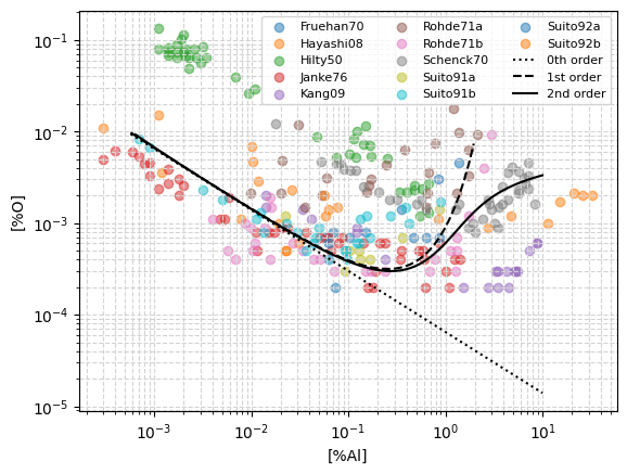
Comparison of equilibrium curves and experimental data#

Below, a comparison of the numerically determined aluminium-oxygen equilibrium curves against experimental data from 12 different sources in the litterature, is presented.

The model results are plotted considering three levels of refinement:

0th order: The interactions between solutes are neglected, this corresponds to setting \(f_{Al} = f_{O} = 1\).
1st order: Only 1st order interactions are considered, this is, only 1st order interaction coefficients are used, \(e_i^j\).
2nd order Both 1st and 2nd order interactions are considered, this is, both 1st and 2nd order interaction parameters are used, \(e_i^j\), \(r_i^j\), \(r_i^{j,k}\).

# Plot using pandas and matplotlib:
T = 1873                            # Temperature, K
pcts = np.logspace(-4, 1, 100)      # Al content range, [%Al]
aAl2O3 = 1                          # Al2O3 activity

fig = plt.figure()
ax = fig.add_subplot(111)

# Plot experimental data
refs = df['Source'].unique()
for ref in refs:
    _df = df[(df['Source'] == ref)]
    ax.scatter(_df['pctAl'], _df['pctO'], marker='o', alpha=0.5, label=ref)
        
# Plot model results
orders = [0, 1, 2]
linestyles = [':', '--', '-']
labels = ['0th order', '1st order', '2nd order']
for order, linestyle, label in zip(orders, linestyles, labels):
    pctM, pctO = data_deox(Al_O_eqs, T, pcts, aAl2O3, x0=1e-8, order=order, bound=1e-2)
    ax.plot(pctM, pctO, ls=linestyle, color='k', label=label)
    
# Make the plot pretty
ax.set_xlabel('[%Al]')
ax.set_ylabel('[%O]')

ax.set_xscale('log')
ax.set_yscale('log')

ax.grid(which='both', ls='--', color='lightgray')

ax.legend(loc='upper right', ncols=3, fontsize=8)
plt.show()

../_images/8c81c5ad32a3f027378d2e7c0f6ff1fc107fce9ce22a18b3bdcd23448cb1f395.png