Fundamentals of steel desulfurization

Fundamentals of steel desulfurization#

Dr. Edgar Ivan Castro Cedeño

import numpy as np
import matplotlib.pyplot as plt
from scipy.integrate import solve_ivp

Metallurgical context#

Generally spearking, sulfur is considered as a nocive element in steel, hence, it is necessary to control it during the steelmaking process

This document focuses on presenting some basic concepts of steel desulfurization, and applying them in studying the process of secondary refining of steel.

Sulfide capacity, Cs.#

The sulfide capacity, \(C_S\), is a widely used concept in pyrometallurgy, the defines the capacity of an homogeneous molten slag for removing sulfur from the bath during the metal refining operations.

It is considered that sulfide capacity is a property that is unique to every slag, and that it depends on its chemical composition and temperature. There exist several models in litterature that allow to estimate sulfide capacity as a function of these paremeters.

The sulfide capacity concept allow to compare under the same workframe, the desulfurization capability of different slag systems.

Measurements of equilibrium sulfur content in slags#

The capability of a slag for dissolving sulfur, \(S^{2-}\), can be determined by means of equilibration experiments between a molten slag and an oxygen-sulfur gas mixture at a fixed temperature. The studied equilibrium reaction is:

\[ \frac{1}{2} S_2(g) + \left(O^{2-}\right)_{slag} = \frac{1}{2} O_2(g) + \left(S^{2-}\right)_{slag} \quad\quad Reac. 1\]

\[ K_1 = \underbrace{\frac{a_{S^{2-}}}{a_{O^{2-}}}}_{non-measurable} \,\,\underbrace{\left(\frac{p_{O_2}}{p_{S_2}}\right)^{1/2}}_{measurable}\]

where \(a_{S^{2-}}\) and \(a_{O^{2-}}\), are the activities of the sulfide and oxygen ions (non-measurable). \(p_{S_2}\) y \(p_{O_2}\), are partial pressures of sulfur and oxygen in the gas mixture (measurable).

Sulfide capacity definition#

Sulfide capacity, as defined by Finchan & Richardson, is obtained after algebraic manipulation of the terms in the equilibrium constant for Reaction 1, in a manner that it can be estimated from measurable quantities.

\[ C_S = \underbrace{K_1 \frac{a_{O^{2-}}}{f_{S^{2-}}}}_{non-measurable} = \underbrace{\left(\%S\right)_{slag} \left(\frac{p_{O_2}}{p_{S_2}}\right)^{1/2}}_{measurable} \]

It is considered that the activity of the sulfide ion is given by: \(a_{S^{2-}} = f_{S^{2-}} \left(\%S\right)_{slag}\).

Modified sulfide capacity, Cs’.#

The modified sulfide capacity, \(C_S'\), is an extension of the sulfide capacity concept, which allows to directly apply it for the case of refining of molten metals and alloys (in this case, steels).

Sulfur exchange reaction between steel and slag#

The sulfur exchange between steel and slag is driven by a ionic reaction at the interface between steel and slag:

\[ \left[ S \right] + \left( O^{2-} \right) = \left( S^{2-} \right) + \left[ O \right] \quad \quad Reac. 2\]

\[ K_2 = \underbrace{\frac{ \left( a_{S^{2-}}\right) }{ \left( a_{O^{2-}}\right) }}_{non-measurable} \,\, \underbrace{\frac{\left[h_O\right] }{\left[h_S\right]}}_{measurable}\]

Modified sulfide capacity definition#

The modified sulfide capacity definition is obtained after algebraic manipulation of the equilibrium constant for Reaction 2.

\[ C_S' = \underbrace{K_2 \frac{a_{O^{2-}}}{f_{S^{2-}}}}_{non-measurable} = \underbrace{\left(\%S\right) \frac{\left[h_O\right]}{\left[h_S\right]}}_{measurable} \]

The activity of the sulfide ion in the slag is given by: \(a_{S^{2-}} = f_{S^{2-}} \left(\%S\right)_{slag}\).

The activities of sulfur and oxygen in the metal are given by: \(h_S = f_S [\%S]\), \(h_O = f_O [\%O]\).

Relating Cs and Cs’#

In order to enable the use of the sulfide capacity concept for estimations of the desulfurizing power of a slag in secondary refining of steel, it is necessary to find the functional relation between \(C_S\), which is obtained from results of equilibrium experiments between molten slags and gas mixtures; and \(C_S'\), which represents the metal processing conditions.

Conversion of the oxygen/sulfur relation, from a ratio of partial pressure to a ratio of solute activities#

The combined reaction of dissolution of oxygen and sulfur in liquid steel is given by:

\[\left[S\right] + \frac{1}{2} \left\{O_2\right\} = \frac{1}{2} \left\{S_2\right\} + \left[O\right] \quad \quad Reac. 3\]

\[K_3 = \frac{\left[h_o\right]}{\left[h_s\right]} \left(\frac{p_{S_2}}{p_{O_2}}\right)^{1/2}\]

Through algebraic manipulation, an expression for the ratio of the oxygen and sulfur activities in the metal is found:

\[\frac{\left[h_o\right]}{\left[h_s\right]} = K_3 \left(\frac{p_{O_2}}{p_{S_2}}\right)^{1/2}\]

Substituting this expression in the definition of \(C_S'\):

\[ C_S' = \underbrace{\left(\%S\right) \left(\frac{p_{O_2}}{p_{S_2}}\right)^{1/2}}_{C_S} K_3\]

According to Andersson, Jönsson & Nzotta, the value of the equilibrium constant for this reaction has the value:

\[\log K_3 = -\frac{935}{T} + 1.375\]

def logK3(T:float) -> float:
    """
    log Equilibrium constant for sulfur-oxygen 
    dissolution reaction (Reac. 3)

    Parameters
    ----------
    T : Float
        Temperature, in [K].
        
    Returns
    -------
        Float
        logarithm base 10 of equilibrium constant for Reac. 3
    """
    return -935.0/T + 1.375

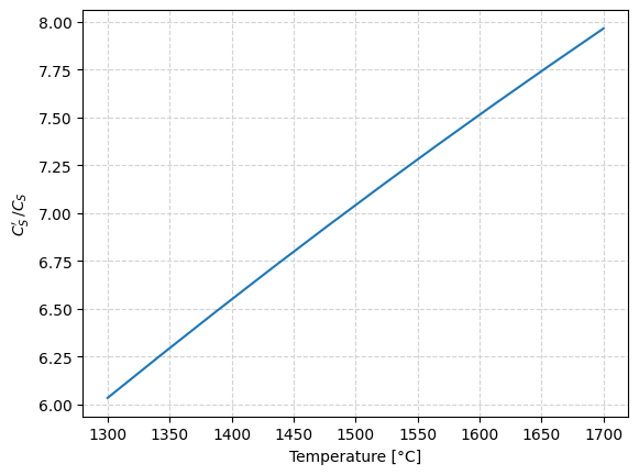
ratio between Cs’ and Cs#

Using the thermodynamic data for Reaction 3, defined in the function logK3(), the plot below is built, which shows the value of the ratio for a range of temperatures between \(1300 \, ^\circ C\) and \(1600 \, ^\circ C\).

fig0 = plt.figure()
ax0 = fig0.add_subplot(111)

Tc0 = np.linspace(1300, 1700, 10)
Tk0 = Tc0 + 273.15

# Plot lines
ratioISIJ0 = np.power(10, logK3(Tk0))
ax0.plot(Tc0, ratioISIJ0)

ax0.set_xlabel("Temperature [°C]")
ax0.set_ylabel(r"$C_S' \, / C_S$")

ax0.grid(ls='--', color='lightgray')

plt.show()

../_images/e4dd11eec2faaddcb72c4f3f87d881e85f513d96d7a370ab442ed95f8738990c.png

Sulfur partition ratio, Ls#

The sulfur partition ratio, \(L_S\), represents the ratio between sulfur contained in the slag and sulfur contained in the metal, under thermodynamic equilibrium conditions.

\[L_S = \frac{(\%S)}{[\%S]} \quad \quad Equilibrio\]

Since measurements of sulfur content in the metal and the slag are relatively easy to perform in the steelshop, it is a commonly used KPI for the steelmaking process. Nevertheless, the metallurgist should remember that steelmaking is a highly transient process, and more often than not the process conditions are out of equilibrium at the time at which sampling is performed.

\[L_{S_{(plant)}} = \frac{(\%S)}{[\%S]} \quad \quad Out \, of \, equilibrium\]

Relation between the sulfur partition ratio and the sulfide capacity#

Starting from the definition of the modified sulfide capacity, and the sulfur activity in the metal, given by \(h_S = f_S [\%S]\), one has:

\[ C_S' = \frac{(\%S)}{[\%S]} \frac{h_O}{f_S} = L_S \frac{h_O}{f_S}\]

Applying logarithm law and reodering the equation a more useful form of the equation is obtained:

\[\log L_S = \log C_S' + \log f_S - \log h_O\]

This equation can also be written in terms of the sulfide capacity, \(C_S\), which are the kind of data that are readily available in the litterature and in models:

\[\log L_S = \log C_S -\frac{935}{T} + 1.375 + \log f_S - \log h_O\]

def logLs(Cs: float, T: float, fs: float, ho:float) -> float:
    """ 
    log of Sulfur partition coefficient Ls
        Ls = (%S)/[%S]

    Parameters
    ----------
    Cs: Float
        Sulfide capacity of the slag, in [wt%]
    T : Float
        Temperature, in [K].
    fs: Float
        Henrian activity coefficient, for sulfur
    ho: Float
        Henrian activity, for oxygen [wt%]
    
    Returns
    -------
        Float
        logarithm base 10 of sulfur partition coefficient
    """
    return np.log10(Cs) + logK3(T) + np.log10(fs) - np.log10(ho)

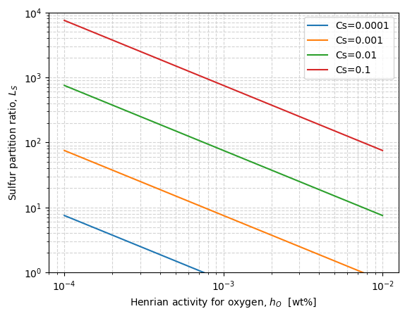
Metallurgical implications#

The equation above allows to put in evidence some strategies to follow in order to maximize the sulfur partition coefficient:

Slag conditioning and temperature control, to obtain a slag with good sulfide capacity, \(C_S\).
Bath deoxidation, to reduce the activity of oxygen in the metal, \(h_O\).

These can be seen when analyzing the function logLs(), defined below, which is plotted for different sulfide capacities, \(C_S\), and oxygen activities, \(h_O\), keeping fixed the temperature \((T = 1600 ^\circ C\)), and the Henrian activity coefficient for sulfur \((f_S = 1)\).

fig1 = plt.figure()
ax1 = fig1.add_subplot(111)

_ao = np.logspace(-4, -2, 10)
_T1 = 1873.15 # 1600 C
_fs = 1

# Plot lines
_CS = np.array([1e-4, 1e-3, 1e-2, 1e-1])

for Cs in _CS:
    _Lsline = np.power(10, logLs(Cs, _T1, _fs, _ao))
    label = "".join(["Cs=", str(Cs)])
    ax1.plot(_ao, _Lsline, label=label)

# Format graph
ax1.set_xscale('log')
ax1.set_yscale('log')
ax1.set_ylim(1, 1e4)

ax1.set_xlabel(r"Henrian activity for oxygen, $h_O$  [wt%]")
ax1.set_ylabel(r"Sulfur partition ratio, $L_S$")


ax1.grid(ls='--', which='both', color='lightgray')
ax1.legend()

plt.show()

../_images/63c5361d5c002f433c5f023ad69cb0b3edb0f5515ac659331f632d7807b74991.png

Effect of slag amount#

Once the metallurgical impact of good slag conditioning \((C_S)\) and bath deoxidation (\(h_O\)), the effect of the slag amounts used in the refining process, \(M_{sl}\) should be quantified. The first step is to perform a stell and slag sulfur mass balance.

Sulfur balance#

The steel-slag sulfur mass balance, normalized per 1000 kg (1 tonne) of steel, is given by:

\[\underbrace{1000 \left[\omega_S\right]_0 + M_{sl} \left(\omega_S\right)_0}_{initial \, state} = \underbrace{1000 \left[\omega_S\right] + M_{sl} \left(\omega_S\right)}_{final \, state} \]

where \(M_{sl}\) is the slag mass given in kg per tonne of steel, \((\omega_S)\) is the mass fraction of sulfur in the slag, and \([\omega_S]\) is the mass fraction of sulfur in the metal.

A common simplified approach consists in neglecting the sulfur contained in the initial slag.

\[\underbrace{1000 \left[\omega_S\right]_0}_{initial \, state} = \underbrace{1000 \left[\omega_S\right] + M_{sl} \left(\omega_S\right)}_{final \, state} \]

Sulfur balance in terms of the partition coefficient and the slag mass#

With some algebraic manipulation the sulfur balance an be rewritten in terms of the sulfur partition coefficient, \(L_S\):

\[1000 \frac{\left[\omega_S\right]_0}{\left[\omega_S\right]} = 1000 + M_{sl} \underbrace{\frac{\left(\omega_S\right)}{\left[\omega_S\right]}}_{L_S} \]

\[\frac{\left[\omega_S\right]_0}{\left[\omega_S\right]} = 1 + \frac{M_{sl}}{1000} L_S \]

This function allows to estimate the sulfur content once the metal=slag equilibrium has been reached, this is, the thermodynamic limit for the desulfurization process.

Ratio of the equilibrium and initial sulfur contents in the metal:

\[\frac{\left[\omega_S \right]}{\left[\omega_S\right]_0} = \frac{1}{1 + \frac{M_{sl}}{1000} L_S} \]

Desulfurization progress once the equilibrium conditions have been reached:

\[R_S = \left(1 - \frac{[\omega_S]}{[\omega_S]_0} \right) \times 100 \%\]

def desulfRatio(Msl: float, Ls: float) -> float:
    """ 
    Ratio of equilibrium and initial sulfur contents in the metal
    as given by a sulfur mass balance.
    
    Parameters
    ----------
    Msl: Float
         kg of molten slag per ton of metal, [kg/ton]
    Ls : Float
         Sulfur partition coefficient, Ls=(%S)/[%S]
    Returns
    -------
        Float
        Ratio of equilibrium and initial sulfur contents in the metal
    """
    return 1 / (1 + (Msl/1000) * Ls)

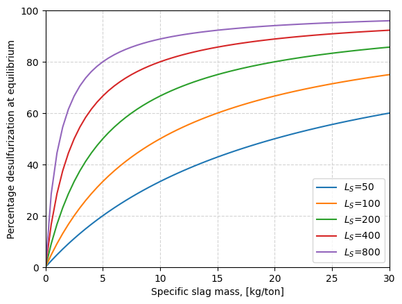
Metallurgical implications#

The equation allows to estimate the maximum desulfurization progress (thermodynamic limit) that is possible in a process for which the slag amount, \(M_{sl}\), and the sulfur partition coefficient, \(L_S\), are known.

The estimations can be seen with the function desulfRatio(), which is plotted for different amounts of slag, \(M_{sl}\) and sulfur partition coefficients, \(L_S\).

fig2 = plt.figure()
ax2 = fig2.add_subplot(111)

_Msl2 = np.linspace(0, 30, 61)

# Plot lines
_Ls2 = np.array([50, 100, 200, 400, 800])

for Ls in _Ls2:
    _pctDesulf = 100 * (1 - desulfRatio(_Msl2, Ls))
    label = "".join([r"$L_S$=", str(Ls)])
    ax2.plot(_Msl2, _pctDesulf, label=label)

# Format graph
ax2.set_ylim(1, 1e4)

ax2.set_xlabel(r"Specific slag mass, [kg/ton]")
ax2.set_xlim(0, 30)
ax2.set_ylabel(r"Percentage desulfurization at equilibrium")
ax2.set_ylim(0, 100)

ax2.grid(ls='--', which='both', color='lightgray')
ax2.legend(loc='lower right')

plt.show()

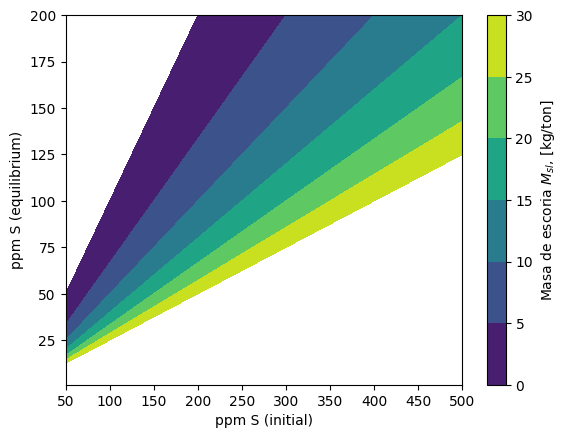
../_images/e60d24379ef9eb5f5c9a7937c26079b2c3e09f7d5f6e26c82b3bfb5585f5e624.png

Starting form the equation of the ratio of sulfur contents, reponse surfaces for the amount of required slag, \(M_{sl}\), for obtaining a given equilibrium sulfur amount \([\omega_S]\), starting from given initial sulfur content, \([\omega_S]_0\), and sulfur partition ratio, \(L_S\).

This calculation is implemented in the function plot_Msl_surf(), which allows to produce the graph shown below.

def Msl_surf(Sini: float, Sfin: float, Ls: float) -> float:
    """
    Masa de escoria [kg/ton] requerida para remocion de azufre
        Sini: Azufre inicial
        Sfin: Azufre final (equilibrio)
        Ls: coeficiente de reparto de azufre
    """
    return 1000/Ls * (Sini/Sfin - 1)

def plot_Msl_surf(Ls:float)->None:
    """
    Grafica la superficie de respuesta de masa de escoria
    requerida para obtener un nivel de azufre en equilibrio
    a partir de un contenido de azufre inicial.
    """
    _Sini = np.linspace(50, 500, 80)
    _Sfin = np.linspace(1, 200, 80)

    X, Y = np.meshgrid(_Sini, _Sfin)
    Z = Msl_surf(X, Y, Ls)

    fig3 = plt.figure()
    ax3 = fig3.add_subplot(111)

    CS3 = ax3.contourf(X, Y, Z, levels=[0, 5, 10, 15, 20, 25, 30])
    cbar3 = fig3.colorbar(CS3, ax=ax3)
    
    ax3.set_xlabel("ppm S (initial)")
    ax3.set_ylabel("ppm S (equilibrium)")
    
    cbar3.ax.set_ylabel(r'Masa de escoria $M_{sl}$, [kg/ton]')
    
    plt.show()

The user is invited to experiment by changing the value of the sulfur partition coefficient in the function plot_Msl_surf()

plot_Msl_surf(Ls = 100)

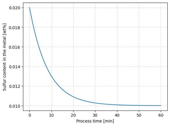
../_images/4e06ae85a9972e818e2a495aea9bfb4dc10670507dd450cd949902883f8cf039.png

Calculation of the desulfurization rate#

As was already mentioned, the desulfurization process is driven by sulfur transfer at the metal-slag interface.

\[ \left[ S \right] + \left( O^{2-} \right) = \left( S^{2-} \right) + \left[ O \right] \quad \quad Reac. 2\]

These kinds of processes can be described by a first order differential equation.

Differential equation for the desulfurization rate#

The first order differential equation that is shown below, allows to estimate the progress of the desulfurization of a steel bath, considering the fact that as sulfur is removed from the metal, the sulfur content in the slag is rising.

\[\frac{d[\%S]}{dt} = -k_{S,emp} \left([\%S] \left(1 + \frac{1}{\frac{M_{sl}}{1000} L_s} \right) - \frac{[\%S_0]}{\frac{M_{sl}}{1000} L_s}\right) \]

Where:

\(k_{S, emp}\): empirical desulfurization constant, characterizing the bath agitation and the extent of the contact area between metal and slag.
\([\%S]\): sulfur content in the metal.
\([\%S_0]\): initial sulfur content in the metal.
\(M_{sl}\): slag amount, in kg/tonne.
\(L_S\): sulfur partition ratio.

def desulfRate(t:float, wS:float, c:float) -> float:
    """
    Desulfurization rate differential equation
    taking into account uptake of sulfur by the slag
    
    Parameters
    ----------
    t : Float
        time, in [s]
    wS: Float
        sulfur content, in [wt%]
    c:  tupple with Floats
        ks: desulfurization rate constant, in [1/s]
        ws0: initial sulfur content in metal, in [wt%]
        Msl: kg of slag per ton of metal, in [kg/ton]
        Ls: sulfur partition coeficient, Ls=(%S)/[%S]
    Returns
    -------
    dwSdt : float
        Desulfurization rate, in [[%S]/s]
    """
    ks, wS0, Msl, Ls = c
    Y = Msl/1000 * Ls
    dwSdt = -ks * (wS * (1 + 1/Y) - wS0/Y)
    return dwSdt

Solution of the differential equation with a numerical method#

Below, a method for the solution of the differential equation written in the function defulfRate(), by using the function solve_ivp, included in the scipy.integrate library, is presented.

The plot_desulfRate() function is used for plotting the results from the numerical integration of the differential equation.

def plot_desulfRate(sol):
    fig = plt.figure()
    ax = fig.add_subplot(111)
    
    t = sol.t/60 # tiempo,[min]
    wS = sol.y[0] # azufre al tiempo t, [wt%]
    
    ax.plot(t, wS)
    ax.set_xlabel("Process time [min]")
    ax.set_ylabel("Sulfur content in the metal [wt%]")
    
    ax.grid(ls='--', color='lightgray')

The user is invited to experiment in order to evaluate the effect of different parameters.

# Define integration time and constants
teval = np.linspace(0, 3600, 121)
ks = 1e-3 # desulfurization constant, [1/s]
wS0 = 0.020 # initial sulfur, [wt%]
Msl = 20 # slag amount, [kg/ton]
Ls = 50 # sulfur partition ratio

# Entries for the solver
tspan = (teval[0], teval[-1])
c = [ks, wS0, Msl, Ls]

# Solve the differential equation
sol = solve_ivp((lambda t, wS: desulfRate(t, wS, c)), t_span=tspan, y0 = [wS0], t_eval=teval)

# plot the result
plot_desulfRate(sol)

../_images/00e6660f2b3381b330db4a476d7bb60228957829c0b90bd462947aa1acadeb75.png

Fundamentals of steel desulfurization

Contents

Fundamentals of steel desulfurization#

Metallurgical context#

Sulfide capacity, Cs.#

Measurements of equilibrium sulfur content in slags#

Sulfide capacity definition#

Modified sulfide capacity, Cs’.#

Sulfur exchange reaction between steel and slag#

Modified sulfide capacity definition#

Relating Cs and Cs’#

Conversion of the oxygen/sulfur relation, from a ratio of partial pressure to a ratio of solute activities#

ratio between Cs’ and Cs#

Sulfur partition ratio, Ls#

Relation between the sulfur partition ratio and the sulfide capacity#

Metallurgical implications#

Effect of slag amount#

Sulfur balance#

Sulfur balance in terms of the partition coefficient and the slag mass#

Metallurgical implications#

Calculation of the desulfurization rate#

Differential equation for the desulfurization rate#

Solution of the differential equation with a numerical method#

Further reading#